The Maxwell‑Boltzmann distribution remains the cornerstone for describing particle speeds in an ideal gas, linking temperature to kinetic energy and enabling accurate predictions in chemistry, physics, and engineering. Recent curriculum updates highlight its relevance for both undergraduate study and industry‑level modelling, prompting educators to emphasize clear visualisations and real‑world examples.
Historical context and theoretical foundation
Developed independently by James Clerk Maxwell (1860) and Ludwig Boltzmann (1872), the distribution emerged from kinetic theory, which treats gases as collections of rapidly moving, non‑interacting particles. By assuming elastic collisions and applying statistical mechanics, the model yields a probability density function that predicts how many particles travel at a given speed at equilibrium.
Key formula and parameters
The probability density f(v) for speed v is expressed as:
- f(v) = 4π ( m / 2πkT )³⁄² v² exp(‑mv² / 2kT)
- m – molecular mass of the gas particle
- k – Boltzmann constant (1.38 × 10⁻²³ J K⁻¹)
- T – absolute temperature (K)
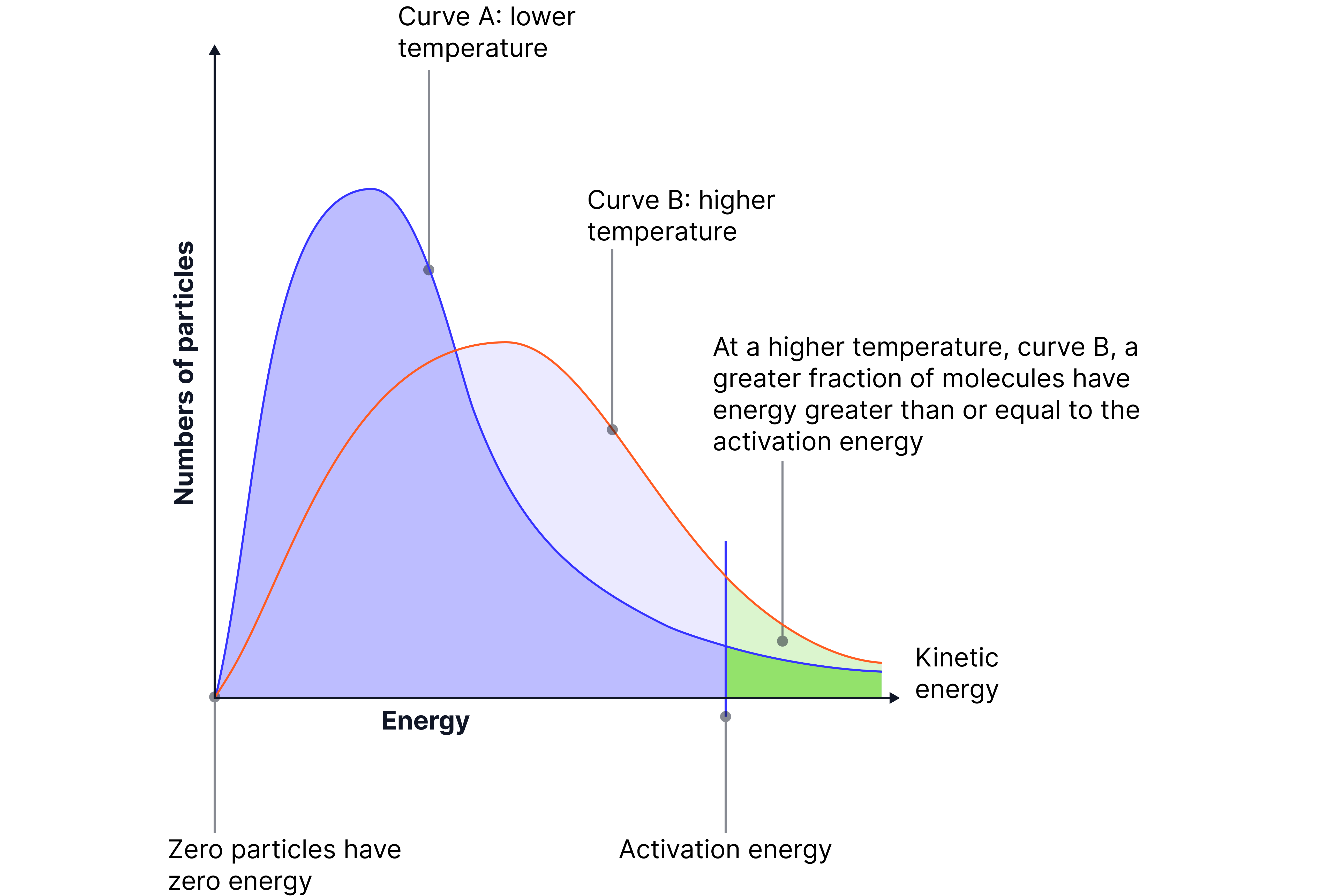
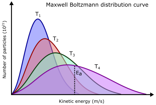
The term v² creates the characteristic bell‑shaped curve, while the exponential factor forces the probability toward zero at very high speeds. As temperature rises, the curve flattens and shifts right, indicating a larger fraction of fast‑moving particles.
Practical applications across disciplines
Understanding the distribution unlocks several everyday and industrial processes:
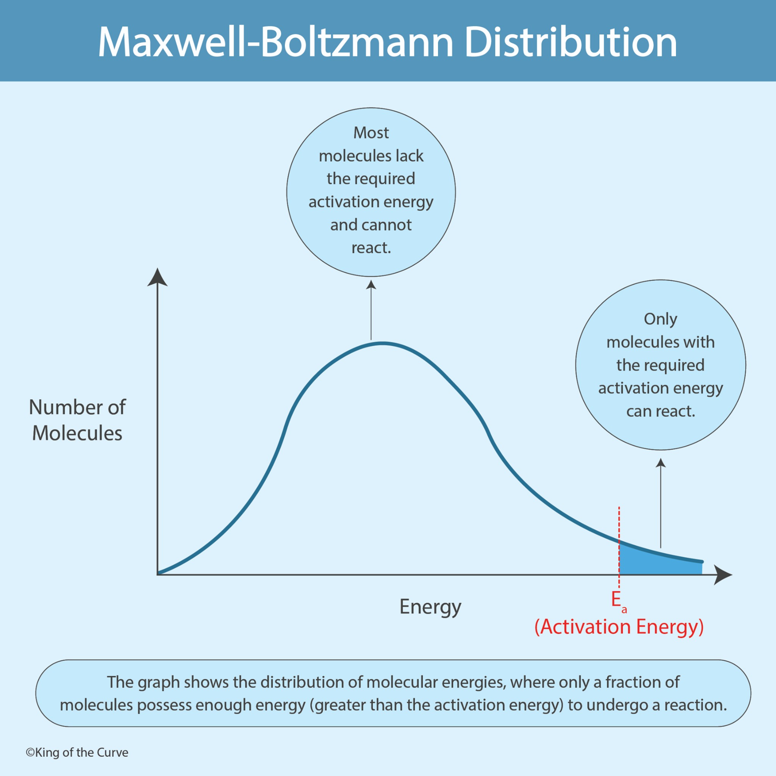
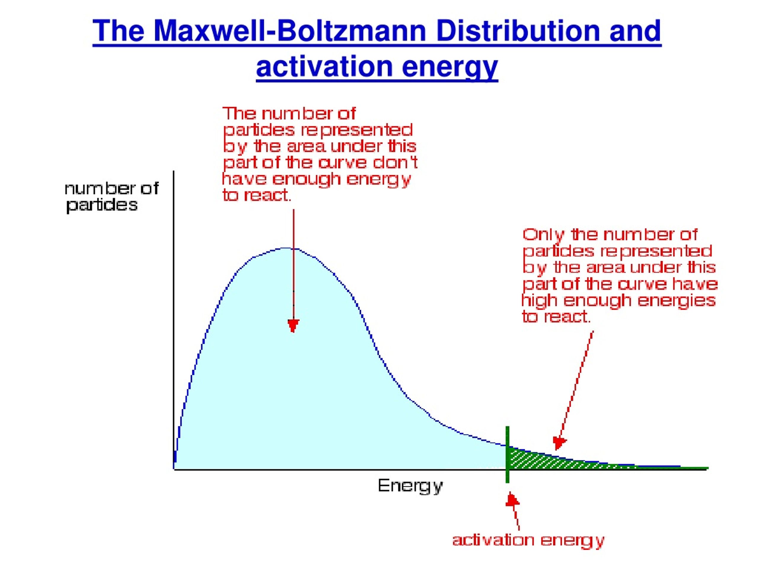
- Reaction rate estimation – Collision theory uses the high‑energy tail of the distribution to calculate the fraction of molecules exceeding activation energy.
- Vacuum system design – Predicting molecular flux through apertures relies on average molecular speed derived from the distribution.
- Aerospace engineering – Atmospheric re‑entry heating models incorporate Maxwell‑Boltzmann statistics to assess gas‑particle impacts on vehicle surfaces.
- Medical imaging – Diffusion‑weighted MRI interprets water‑molecule speed distributions to infer tissue microstructure.
Common misconceptions addressed
Students often conflate the Maxwell‑Boltzmann curve with a normal distribution. Unlike a true Gaussian, the speed distribution is bounded at zero and exhibits a skewed shape that depends on temperature. Additionally, the model assumes ideal behaviour; real gases deviate at high pressures, where intermolecular forces become significant.
Integrating the distribution into classroom instruction
Effective teaching blends analytical derivation with visual tools. The image below, sourced from a leading educational platform, illustrates how the curve evolves with temperature, offering a quick reference for problem‑solving sessions.

Guided labs that measure gas pressure and temperature, then compare experimental speed data to the theoretical curve, reinforce the link between abstract formulae and tangible outcomes. Providing students with spreadsheet templates to plot f(v) for varying T and m encourages independent exploration.
Future outlook
Advances in computational chemistry increasingly embed the Maxwell‑Boltzmann distribution within molecular dynamics simulations, improving accuracy for reaction‑pathway predictions. As interdisciplinary curricula grow, the ability to translate speed statistics into actionable design criteria will remain a valuable skill for graduates entering research, manufacturing, or technology sectors.
🧪 Maxwell–Boltzmann Distribution: Understanding Molecular Energy In
🧪 Maxwell–Boltzmann Distribution: Understanding Molecular Energy in ...
Answered: The Maxwell -Boltzmann Distribution Of… | Bartleby

Answered: The Maxwell -Boltzmann distribution of… | bartleby
PPT - Factors Affecting Chemical Reaction Rate: Concentration
PPT - Factors Affecting Chemical Reaction Rate: Concentration ...
Maxwell Boltzmann Distribution Read The Question Carefully And Answer
Maxwell Boltzmann Distribution Read The Question Carefully And Answer